

Welcome to the eodc Blog! This is where we’ll share service and product updates, new datasets, tutorials, and stories from the Earth Observation (EO) community. And we couldn’t think of a better way to start than with eodc Orbit.
Your new gateway to everything eodc
On a mission to create a better place to discover and access EO data, eodc developed Orbit, replacing the existing eodc Portal while maintaining the data and services found there. Along the way, Orbit became something bigger: the entry point to all eodc services. With Orbit, you can see everything we offer, explore data before starting your analysis, and get straight into the tools you need.
Here’s an overview of what you’ll find there.
One data catalogue
At the heart of Orbit is a single data catalogue. It brings together the analysis-ready data we host at eodc as well as data from external sources, connected through a federated system. Everything is described with STAC-compliant metadata, so it’s consistent to search and easy to use in your own application.
What it includes:
• Satellite mission data: Derived from Copernicus Sentinel, NASA, and other missions
• Austrian and global datasets: National and international weather, climate, and terrain data
• Variety of data formats: Data is available in GeoTIFF, COG, netCDF and further formats, with a growing focus on Zarr (GeoZarr)

Explore data before starting your analysis
EO datasets can be massive. Instead of bringing the data to you, Orbit brings you to the data. Cloud-native formats like Zarr and Cloud-Optimized GeoTIFF (COG) make this possible by letting you read only the parts you need, straight from where the data is stored. Orbit’s explorers build on this: check whether a dataset covers your area, time range or variable, inspect, slice and visualise it in your browser, and run your analysis right next to the data.
Zarr Explorer
Zarr Explorer lets you work with datacubes interactively. In a few clicks you can:
• Slice data in time
• Plot time series for a location
• Compute time averages
• Stack layers to create true- and false-colour images
Step 1. Overview
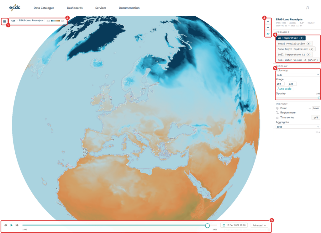
The map fills most of the screen. The menu button (1) opens the list of datasets. Next to it, the name of the dataset and its colour scale (2) show what you are looking at. Use the zoom buttons (3) to move closer. The 2D button next to them switches between the globe and a flat map. On the right (4), choose which variable to show and how it looks. Under the display menu (5), change the colour map, the value range, and the opacity. The time selector (6) at the bottom sets the date.
You should see a map coloured by the data, the dataset name in the top-left corner, and the time selector at the bottom.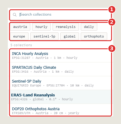
Step 2. Choose a dataset
Click the menu button. Type in the search field (1), or click the filter buttons (2), to narrow the list. The number under the filters says how many datasets match. Click a dataset in the list (3) to open it. The dataset you are viewing is highlighted. Press Esc to close the menu without choosing.
You should see the map and the panel on the right switch to the dataset you chose.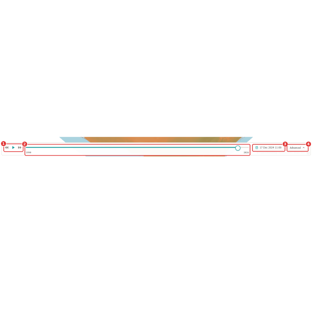
Step 3. Pick a date
The arrows and the play button (1) move through time one day at a time. The slider (2) covers the whole record: click it, or drag the round handle, to jump to a date. The date (3) shows the day you are looking at; click it to choose another one from a calendar. Advanced (4) opens more controls, described in Step 5.
You should see the map redraw for the date you pick.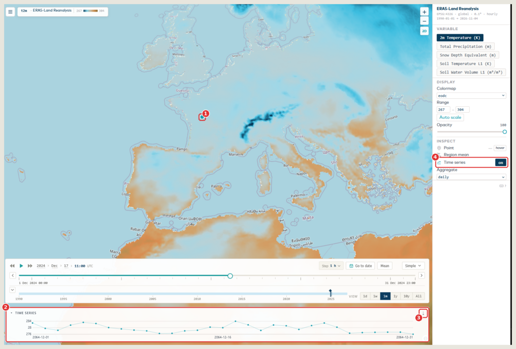
Step 4. Look at one place over time
Click anywhere on the map. A marker (1) shows your point, and the time series (2) at the bottom shows the values at that point over time. The arrow (3) at the right of the chart title saves the values. If no chart appears, check that Time series (4) is switched on in the right-hand panel.
Here the advanced slider is open, so the chart shows one month. With the simple selector it shows the whole record.
You should see the marker on the map and a line chart with the values at that point.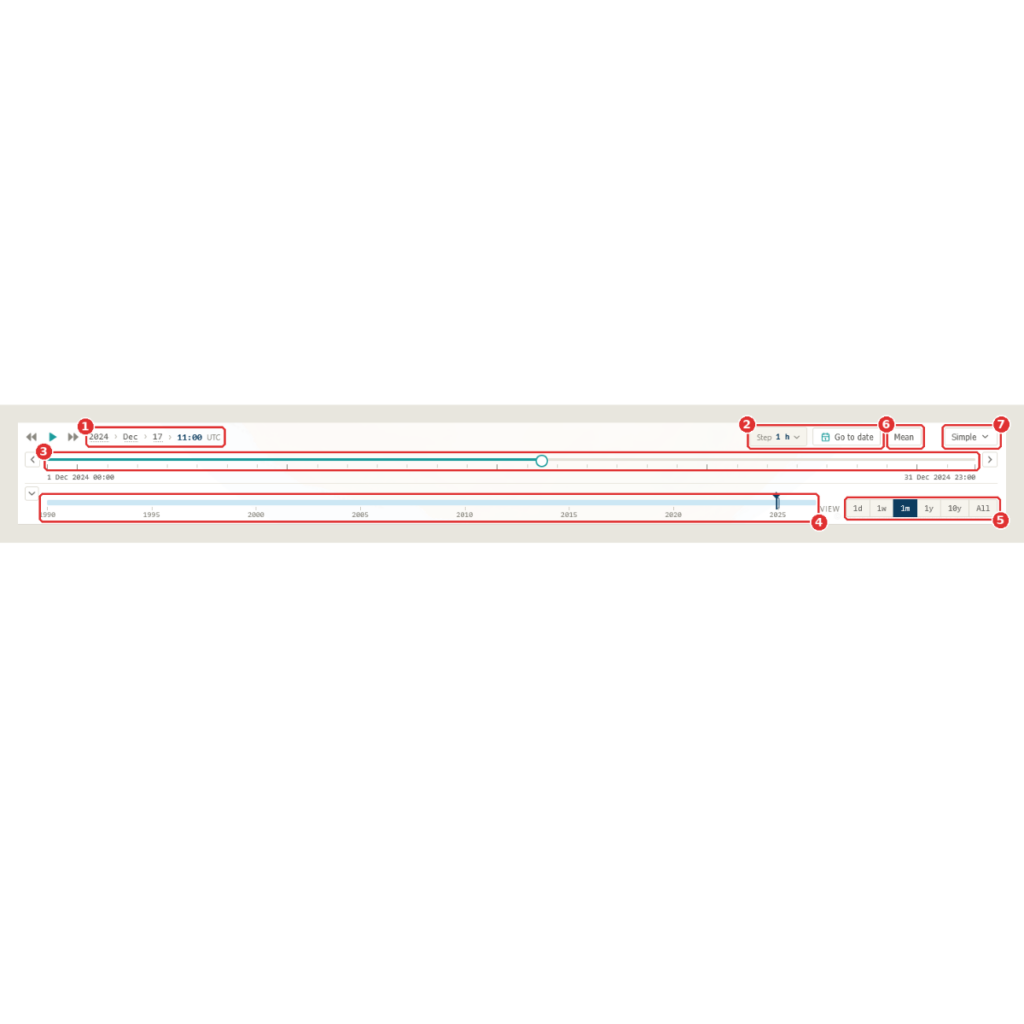
Step 5. Zoom into a period with the advanced slider
Click Advanced to open the full slider. The top row shows the date you are at (1). Next to it you can set how far each step moves with Step, or jump straight to a date with Go to date (2). The upper bar (3) shows one period, for example one month: click it, or drag the round handle, to move through it. The arrows at its ends move to the previous or next period. The lower bar (4) shows the whole record: click it to move to another period. The View buttons (5) set the length of the period: one day, one week, one month, one year, ten years or all. Mean (6) is explained in the next step. Simple (7) takes you back to the simple selector.
You should see two bars: one for the current period and one for the whole record.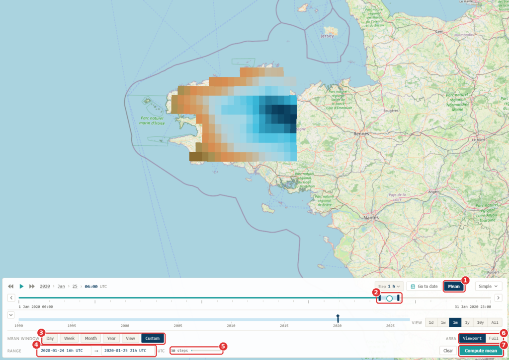
Step 6. Average over a period
Switch on Mean (1). A light-blue band with two dark handles (2) appears on the upper bar and marks the period to average. Choose its length with the buttons (3), or type the start and the end in the Range fields (4). The number next to them (5) shows how many time steps will be averaged. Area (6) chooses how much of the map is averaged: the part you can see (Viewport) or all of it (Full). Press Compute mean (7) to calculate it. Clear, next to it, removes the result.
You should see the map change to show the average over your period.


STAC Explorer
STAC Explorer is built to find the right data quickly. It allows you to:
• Search and filter eodc-hosted collections stored as Cloud-Optimised GeoTIFFs
• Preview individual items live at full resolution
• Copy a ready-made code snippet to keep working in Python.
Step 1. Overview
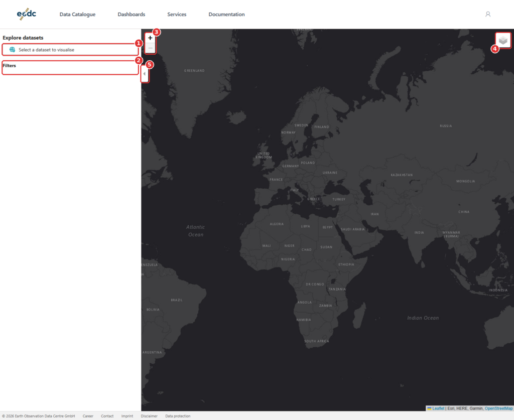
The panel on the left is where you search and browse. The map on the right shows what you find. Click Select a dataset to visualise (1) to begin. The Filters area (2) fills in after you pick a dataset. Use the zoom buttons (3) and the layers button (4) to change the map, and the small arrow (5) to fold the panel in and out.
You should see a side panel and a dark world map.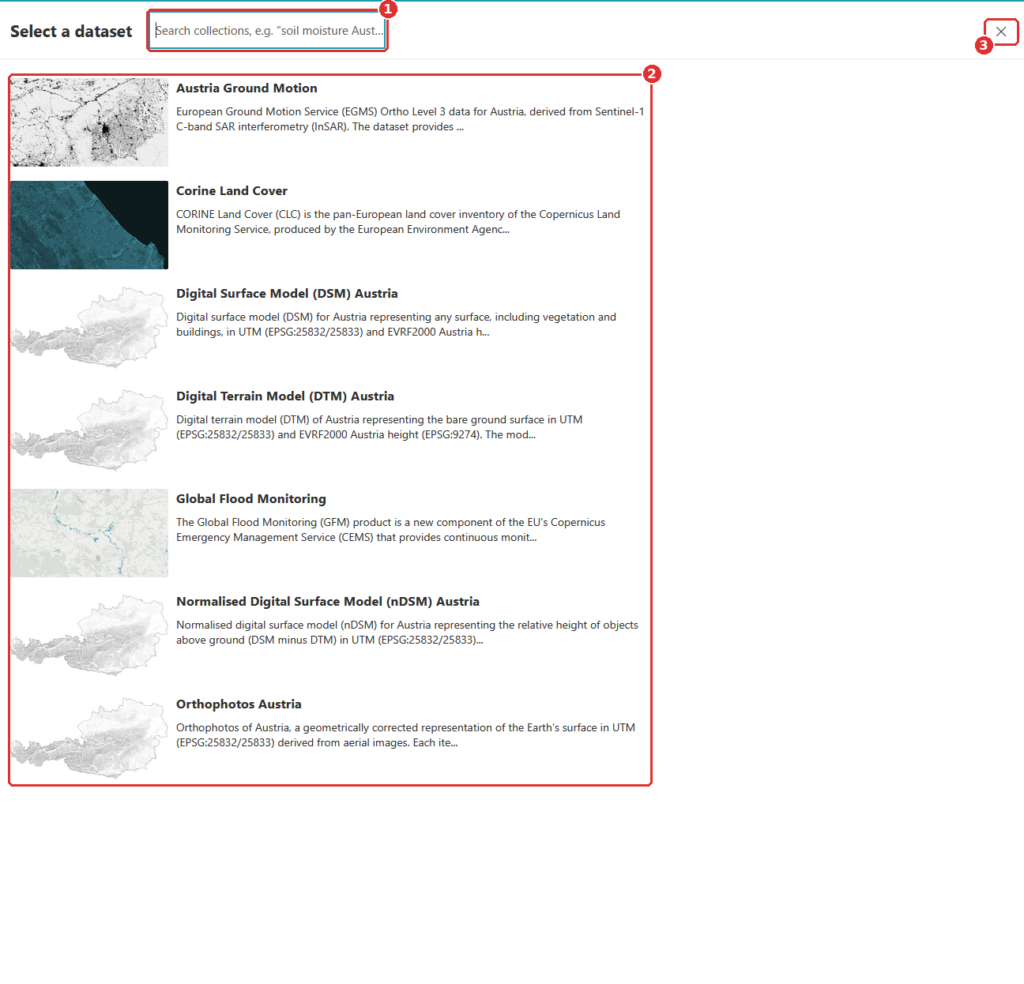
Step 2. Choose a dataset
A list of datasets opens. Type a few words in the search field (1), for example a topic or a place, or scroll the list (2). Click a dataset to select it. The cross (3) closes the list without choosing.
You should see the list of datasets. Typing in the search field narrows it down.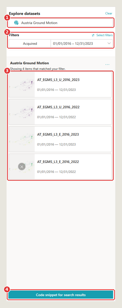
Step 3. Narrow down the results
The dataset you chose is shown at the top (1); Clear next to it removes it. Under Filters (2) you can limit the results by acquisition date, here 1 January 2016 to 31 December 2023. Below that, the results (3) list every item that matches, one card each, with a preview, the item’s ID and its dates. Code snippet for search results (4) gives you Python code that repeats this search.
You should see how many items matched, with one card per item.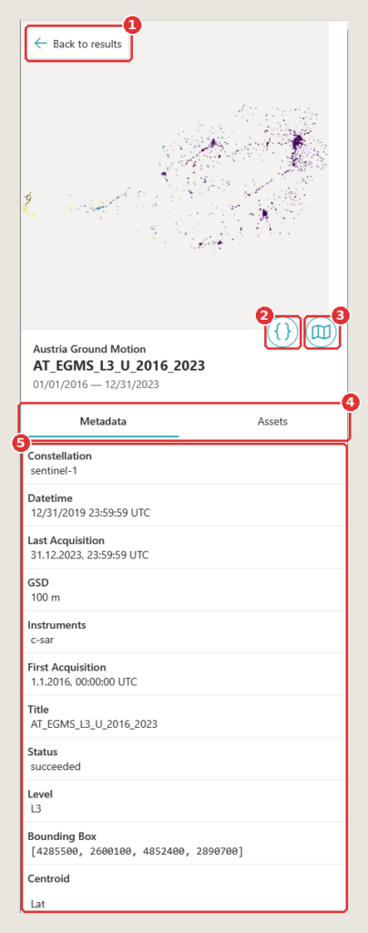
Step 4. Open an item
Click a result to open it. Back to results (1) returns to the list. The { } button (2) shows code for this item, and the map button (3) shows the item on the map. The tabs (4) switch between Metadata and Assets, the item’s data files. The metadata (5) lists facts such as the satellite constellation, the instruments, the resolution (GSD) and the bounding box.
You should see the item’s name, its dates and its metadata.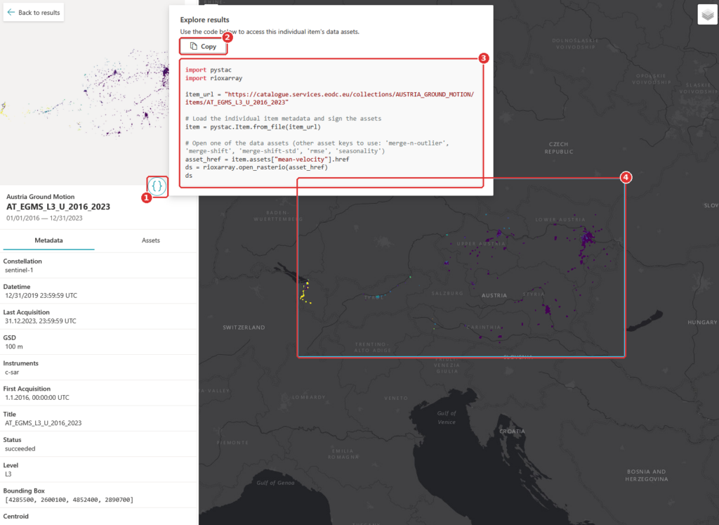
Step 5. Copy the code
Click { } (1). A window opens with Python code for this item. Copy (2) copies it. The code (3) uses the packages pystac and rioxarray to open one of the item’s data files. The blue frame (4) marks the item on the map. Paste the code into a notebook or a script to start working with the data.
You should see a window with Python code, and the item marked on the map.


Dashboards, ready to use
Some questions are best answered with a purpose-built app. eodc Orbit includes ready-to-use dashboards, including:
• S1 Map: Explore our Sentinel-1 SAR Global Backscatter model on an interactive map
• Equi7Grid viewer: See how the Equi7Grid tiles the globe and find the tiles you need, which makes working with the grid much easier
• Flood Events: View the largest 100 flood events since 2015, with interactive visualisation
The dashboard gallery will keep growing as we add further apps. Keep an eye out on eodc’s channels to know when more dashboards are added.
All our services in one place
Orbit’s service catalogue gives you a complete overview of what eodc offers, so you can see what’s available and get started without hunting through separate pages. It includes:
• JupyterHub for interactive analysis in notebooks
• Dask Gateway for scaling your computations
• STAC API for programmatic data search
• OGC APIs via pygeoapi
• TiTiler for dynamic map tiles
• Customer-managed STAC
• Cloud Computing on eodc’s OpenStack cloud
• High-Performance Computing on Austrian Scientific Computing systems
• Object Storage that is S3-compatible and managed yourself

New: Customer-managed STAC
With customer-managed STAC, organisations can host their own STAC catalogues at eodc and decide exactly who can see them. Keep a catalogue private to your team, share it with selected partners, or make it available more widely. Your data sits alongside the eodc catalogue and compute services, using the same standards.
Support when you need it
Every service in Orbit is backed by documentation in the eodc Knowledgebase. You’ll find how-to guides, service documentation, and example notebooks you can run and adapt for your own work.
For organisations, Orbit will also change how access works. In the future, organisation admins will be able to manage which services their users can access, directly in Orbit, without a round of emails to our support team.
To stay up to date on the latest updates, subscribe to our mailing list.
Get started
Getting started is easy: simply open Orbit and start browsing the catalogue, the explorer, and the dashboards right away. Find more information here.
Note that some services require you to sign in. To take full advantage of these services, register for an EODC account at: eodc.eu/register.
We built Orbit to make working with EO data simpler, and we’d love to hear how it works for you. Have a look around and send us your thoughts at feedback@eodc.eu.